Lesson 4 P2 - FastAI


path = untar_data(URLs.MNIST_SAMPLE)  #path for data
Path.BASE_PATH = path


threes = (path/'train'/'3').ls().sorted() #getting 3's data from path
sevens = (path/'train'/'7').ls().sorted() #getting 7's data from path

seven_tensors = [tensor(Image.open(o)) for o in sevens]
three_tensors = [tensor(Image.open(o)) for o in threes]

stacked_sevens = torch.stack(seven_tensors).float()/255
stacked_threes = torch.stack(three_tensors).float()/255
valid_3_tens = torch.stack([tensor(Image.open(o))
                            for o in (path/'valid'/'3').ls()])
valid_3_tens = valid_3_tens.float()/255


valid_7_tens = torch.stack([tensor(Image.open(o))
                            for o in (path/'valid'/'7').ls()])
valid_7_tens = valid_7_tens.float()/255
train_x = torch.cat([stacked_threes, stacked_sevens]).view(-1, 28*28) #.view reshapes the image where each row has 1 image
                                                                    # with all its content in a single row (each image is 28x28)
train_y = tensor([1]*len(threes) + [0]*len(sevens)).unsqueeze(1)
train_x.shape,train_y.shape
dset = list(zip(train_x,train_y)) #zip() creates a concatination of x,y
x,y = dset[0]
x.shape,y
valid_x = torch.cat([valid_3_tens, valid_7_tens]).view(-1, 28*28)
valid_y = tensor([1]*len(valid_3_tens) + [0]*len(valid_7_tens)).unsqueeze(1)
valid_dset = list(zip(valid_x,valid_y))
def init_params(size, var=1.0): return (torch.randn(size)*var).requires_grad_()
weights = init_params((28*28,1)) #weights needed for every pixel, hence 28*28
bias = init_params(1) #Need bias because w*p = 0 when p=0 (p = pixel)
(train_x[0]*weights.T).sum() + bias #Must transpose so multi can happen
def linear1(xb):
    return xb@weights + bias #@ repersents matrix multi

preds = linear1(train_x)
preds #preds of all images
def sigmoid(x): return 1/(1+torch.exp(-x))
plot_function(torch.sigmoid, title='Sigmoid', min=-4, max=4)

def mnist_loss(predictions, targets):
    predictions = predictions.sigmoid() #squishing predictions between 0-1
    return torch.where(targets==1, 1-predictions, predictions).mean()
coll = range(15)
dl = DataLoader(coll, batch_size=5, shuffle=True) #creates minibatches
list(dl)
ds = L(enumerate(string.ascii_lowercase))
ds
dl = DataLoader(ds, batch_size=6, shuffle=True)  #Works with tuples as well
list(dl)
batch = train_x[:4]
batch.shape
linear1??
preds = linear1(batch) #Get pred (initialize weights)
preds
loss = mnist_loss(preds, train_y[:4])
loss
mnist_loss??
loss.backward()
weights.grad.shape, weights.grad.mean(), bias.grad
def calc_grad(xb, yb, model):
    preds = model(xb)
    loss = mnist_loss(preds, yb)
    loss.backward()
def train_epoch(model, lr, params):
    for xb,yb in dl: #get x and y batch
        calc_grad(xb, yb, model) #Calc grad

        for p in params:
            p.data -= p.grad*lr #Update/take a step
            p.grad.zero_() #Set grad to zero
(preds>0.0).float() == train_y[:4]
def batch_accuracy(xb, yb):
    preds = xb.sigmoid()
    correct = (preds>0.5).float() == yb  #.5 because sigmoid(0) = .5
    return correct.float().mean()
batch_accuracy(linear1(batch), train_y[:4])
def validate_epoch(model):
    accs = [batch_accuracy(model(xb), yb) for xb,yb in valid_dl]
    return round(torch.stack(accs).mean().item(), 4)
validate_epoch(linear1)
weights = init_params((28*28,1))
bias = init_params(1)
dl = DataLoader(dset, batch_size=256) #create minibatches

#We can grab the first batch and take a look at it
xb,yb = first(dl)
xb.shape,yb.shape
valid_dl = DataLoader(valid_dset, batch_size=256) #Create minibatch for validation set
lr = 1.
params = weights,bias
train_epoch(linear1, lr, params)
validate_epoch(linear1)
for i in range(20):
    train_epoch(linear1, lr, params)
    print(validate_epoch(linear1))
Congratulation you have created ur official ML model from scratch!
linear_model = nn.Linear(28*28,1) #Does exactly what out funtion linear1 does and initialzes our parameters for us
w,b = linear_model.parameters()
w.shape,b.shape
class BasicOptim:
    def __init__(self,params,lr):
        self.params = list(params)
        self.lr = lr

    def step(self, *args, **kwargs):
        for p in self.params:
            p.data -= p.grad.data * self.lr

    def zero_grad(self, *args, **kwargs):
        for p in self.params:
            p.grad = None
opt = BasicOptim(linear_model.parameters(), lr)
def train_epoch(model):
    for xb,yb in dl:
        calc_grad(xb, yb, model)
        opt.step()
        opt.zero_grad()
validate_epoch(linear_model)
def train_model(model, epochs):
    for i in range(epochs):
        train_epoch(model)
        print(validate_epoch(model), end=' ')
train_model(linear_model, 20)
linear_model = nn.Linear(28*28,1) #fastAI
opt = SGD(linear_model.parameters(), lr) #fastAI
train_model(linear_model, 20)
dls = DataLoaders(dl, valid_dl) #NOT dataLoader, this class stores away the train and valid data into a single obj
learn = Learner(dls, nn.Linear(28*28,1), opt_func=SGD,
                loss_func=mnist_loss, metrics=batch_accuracy)
learn.fit(10, lr=lr)
I hope you now feel comfortable creating from scratch as well as using FastAI ToolKit where possible
Adding a Nonlinearity
We can improve our model by adding some nonlinearity to it. So far we have been using a simple linear classifier. A linear classifier is very constrained. To make it a perform better, we need to add something nonlinear between two linear classifiers—this is what gives us a neural network.
def simple_net(xb):
    res = xb@w1 + b1 #Linear func
    res = res.max(tensor(0.0)) #Activation func: ReLU
    res = res@w2 + b2 #Linear func
    return res
This is all you need to change to implement nonlinearity. Before we were using linear1. Compare this to that.
w1 = init_params((28*28,30))
b1 = init_params(30)
w2 = init_params((30,1))
b2 = init_params(1)
plot_function(F.relu)

simple_net = nn.Sequential(
    nn.Linear(28*28,30), #30 sets of weights
    nn.ReLU(),
    nn.Linear(30,1) #convert back into 1 set of weights
)
learn = Learner(dls, simple_net, opt_func=SGD,
                loss_func=mnist_loss, metrics=batch_accuracy)
learn.fit(40, 0.1)
plt.plot(L(learn.recorder.values).itemgot(2));

m = learn.model
m
w, b = m[0].parameters()
w.shape
w[0].view(28,28)
show_image(w[2].view(28,28))

Seems like this neuron was looking for curves
dls = ImageDataLoaders.from_folder(path)
learn = cnn_learner(dls, resnet18, pretrained=False,
                    loss_func=F.cross_entropy, metrics=accuracy)
learn.fit_one_cycle(1, 0.1)

#Thats insane
Out preformed our model in a single epoch! Guess we still have a lot more to learn :)
- How is a grayscale image represented on a computer? How about a color image?
Image on the computer are represented by a number value, where 0=white, 255=black, and the grayscale inbetween.
A grayscale image is rank 2 (No color channels)
A color image is rank 3 (Has the 3 color channels, RGB) - How are the files and folders in the
MNIST_SAMPLEdataset structured? Why?
Files are split into train, valid, labels. This makes it easier as the training and validation set have already been presplit for for. - Explain how the "pixel similarity" approach to classifying digits works.
This is similer to the Nearest neighbors approach, where one compare each test image with all training images. Only here, the image being compared to is an average of all the training images. Then using a distance metric we can find the abs difference between the images to identify it. - What is a list comprehension? Create one now that selects odd numbers from a list and doubles them. A python condensing technique used with for-loop.
l = [i for i in range(20)]
oddList = [i**2 for i in l if i%2 != 0]
- What is a "rank-3 tensor"?
A 3 dimensional tensor (Also known as a volumn). What is the difference between tensor rank and shape? How do you get the rank from the shape?
Rank refers to the number of dimensions in a tensor
Shape is the size of each dimension of a tensorTaking the len(shape) = rank
- What are RMSE and L1 norm?
Loss functions - How can you apply a calculation on thousands of numbers at once, many thousands of times faster than a Python loop?
Broadcasting - Create a 3×3 tensor or array containing the numbers from 1 to 9. Double it. Select the bottom-right four numbers.
t = tensor(list(range(1,10))).view(3,3)
t[1:,0:2]
- What is broadcasting?
A technique of applying an operation onto all values within an object, often, regardless of tensor (Exceptions do apply). - Are metrics generally calculated using the training set, or the validation set? Why?
Validation set as it contains unseen data. - What is SGD?
Optimization algorithm. This is what causes the loss to decrease as it steps/updates the parameters. - Why does SGD use mini-batches?
Minibatches are faster and more efficient on GPU. Also, they gradient is calculated more appropriately as doing it across the entire batch could cause unstable and imprecise gradients. - What are the seven steps in SGD for machine learning?
Initialize parameters
Compute perdiction
Get loss
Get gradients
Update wieghts
Repeat
Stop - How do we initialize the weights in a model?
Randomly - What is "loss"?
A metric used by the computer to determine its performance - Why can't we always use a high learning rate?
Stepping to far can cause the model to increase loss or bounce and diverge - What is a "gradient"?
Slope. This tell us how much we have to change each weight to make our model better. - Do you need to know how to calculate gradients yourself?
No - Why can't we use accuracy as a loss function?
A loss function needs to change as the weights are being adjusted. Accuracy only changes if the predictions of the model changes. - Draw the sigmoid function. What is special about its shape?
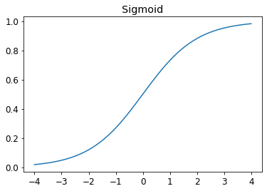
Squishes all values between 0-1 - What is the difference between a loss function and a metric?
The loss function is understood by the computer, while a metric is understood by us humans. - What is the function to calculate new weights using a learning rate?
The optimizer step function (Ex: SGD). - What does the
DataLoaderclass do?
Creates minibatches Write pseudocode showing the basic steps taken in each epoch for SGD.
for x,y in data:
 pred = model(x)
 loss = loss_func(pred, y)
 loss.backward()

 for p in self.params:
     p -= parameters.grad * lr
     p.grad = None
- Create a function that, if passed two arguments
[1,2,3,4]and'abcd', returns[(1, 'a'), (2, 'b'), (3, 'c'), (4, 'd')]. What is special about that output data structure?def func(l1,l2): return list(zip(l1,l2))
- What does
viewdo in PyTorch?
Reshapes tensor - What are the "bias" parameters in a neural network? Why do we need them?
So that the gradient isnt set to 0 during the first iteration. - What does the
@operator do in Python?
Matrix multi - What does the
backwardmethod do?
Calculated gradients - Why do we have to zero the gradients?
PyTorch remembers the previously stored gradients - What information do we have to pass to
Learner?
dataset (DataLoaders), model (Ex: nn.Linear), opt func (Ex: SGD), loss func (Ex: mnist_loss), metric(Optional) Show Python or pseudocode for the basic steps of a training loop.
def train_epoch(model,lr,params):
     for x,y in dl:
         calc_grad(x,y,model)

     for p in self.params:
         p -= parameters.grad * lr
         p.grad = None

 for i in range(epochs):
     train_epoch(model, lr, params)
What is "ReLU"? Draw a plot of it for values from
-2to+2.
Activation function- What is an "activation function"?
The purpose of an activation function is to add non-linearity to the model. - What's the difference between
F.reluandnn.ReLU?
F.relu is a Python function nn.ReLU is a PyTorch module (So part of a class) - The universal approximation theorem shows that any function can be approximated as closely as needed using just one nonlinearity. So why do we normally use more?
There are performance benefits to using more than one nonlinearity
- Create your own implementation of
Learnerfrom scratch, based on the training loop shown in this chapter. - Complete all the steps in this chapter using the full MNIST datasets (that is, for all digits, not just 3s and 7s). This is a significant project and will take you quite a bit of time to complete! You'll need to do some of your own research to figure out how to overcome some obstacles you'll meet on the way.
Completed, see here: https://usama280.github.io/PasteBlogs/