Lesson 9 - FastAI


from fastbook import *
from kaggle import api
from pandas.api.types import is_string_dtype, is_numeric_dtype, is_categorical_dtype
from fastai.tabular.all import *
from sklearn.ensemble import RandomForestRegressor
from sklearn.tree import DecisionTreeRegressor
from dtreeviz.trees import *
from IPython.display import Image, display_svg, SVG

pd.options.display.max_rows = 20
pd.options.display.max_columns = 8
!echo '{"username":"unadeem","key":"ed1df5a2cd97f9d82e42c37511c02095"}' > /root/.kaggle/kaggle.json
!kaggle competitions download -c bluebook-for-bulldozers #Downloading data from Kaggle
import zipfile

z= zipfile.ZipFile('bluebook-for-bulldozers.zip') #unzip first
z.extractall() #extract
df = pd.read_csv('TrainAndValid.csv', low_memory=False) #get data from csv file
df.columns
df['ProductSize'].unique() #Lets view this oridnal colomn
Notice that these seem to be in random order, we should fix this as order has value
sizes = 'Large','Large / Medium','Medium','Small','Mini','Compact' #our desired order
df['ProductSize'] = df['ProductSize'].astype('category') #Turn into categorical variable

df['ProductSize'].cat.set_categories(sizes, ordered=True, inplace=True) #Now we can set our order
df['ProductSize'].unique()
dep_var = 'SalePrice' #our label
df[dep_var] = np.log(df[dep_var]) #kaggle wants us to do MNSLE, so we must take log
We actually don't know how to come up with these question, so we have the model do it for us!
df = add_datepart(df, 'saledate')
' '.join(o for o in df.columns if o.startswith('sale'))
Notice the many distinct categories
df_test = pd.read_csv(Path()/'Test.csv', low_memory=False)
df_test = add_datepart(df_test, 'saledate') #Doing the same for test dataset
Using TabularPandas and TabularProc
We actually need to clean our data a little more. Will be using a transform, TabularProc: Specifically Categorify and FillMissing. Categorify replaces columns with numerical categorical columns, and FillMissing replaces missing values with the median of the column.
procs = [Categorify, FillMissing]
cond = (df.saleYear<2011) | (df.saleMonth<10)
train_idx = np.where( cond)[0]
valid_idx = np.where(~cond)[0]

splits = (list(train_idx),list(valid_idx))
len(cond), len(train_idx), len(valid_idx)
cont,cat = cont_cat_split(df, 1, dep_var=dep_var) #Also pass our label so it isnt included
cont[:4]
cat[:4]
to = TabularPandas(df, procs, cat, cont, y_names=dep_var, splits=splits)
len(to.train),len(to.valid)
to.show(3) #We can view our data similer to DataLoader
to.items.head(3)
to1 = TabularPandas(df, procs, ['state', 'ProductGroup', 'Drive_System', 'Enclosure'], [], y_names=dep_var, splits=splits)
to1.show(3)
It shows strings, but it's actually stored internally as digits. See below:
to1.items[['state', 'ProductGroup', 'Drive_System', 'Enclosure']].head(3)
These values are referring to the vocab
to.classes['ProductSize']
save_pickle(Path()/'to.pkl',to)
Lets also export what we currently have, so we don't have to rerun the processing
xs,y = to.train.xs,to.train.y
valid_xs,valid_y = to.valid.xs,to.valid.y
m = DecisionTreeRegressor(max_leaf_nodes=4) #Creating tree
m.fit(xs, y) #Fitting
draw_tree(m, xs, size=10, leaves_parallel=True, precision=2)
We can also view the above information using another library
samp_idx = np.random.permutation(len(y))[:500]
dtreeviz(m, xs.iloc[samp_idx], y.iloc[samp_idx], xs.columns, 'SalePrice',
        fontname='DejaVu Sans', scale=1.6, label_fontsize=10,
        orientation='LR')
Notice that here we can see that their are models made in the 1000's which is obv not true:We can fix this
xs.loc[xs['YearMade']<1900, 'YearMade'] = 1950
valid_xs.loc[valid_xs['YearMade']<1900, 'YearMade'] = 1950
m = DecisionTreeRegressor(max_leaf_nodes=4).fit(xs, y)

dtreeviz(m, xs.iloc[samp_idx], y.iloc[samp_idx], xs.columns, 'SalePrice',
        fontname='DejaVu Sans', scale=1.6, label_fontsize=10,
        orientation='LR')
Now it looks a little cleaner
m = DecisionTreeRegressor()
m.fit(xs, y);
def r_mse(pred,y): return round(math.sqrt(((pred-y)**2).mean()), 6)
def m_rmse(m, xs, y): return r_mse(m.predict(xs), y)
m_rmse(m, xs, y)
We got 0! Does that mean our model is perfect? No, as you will see below the validation performs worse. We are overfitting.
m_rmse(m, valid_xs, valid_y)
m.get_n_leaves(), len(xs) #lets view how many leaves we have
We seem to have just as much leave nodes as data
m = DecisionTreeRegressor(min_samples_leaf=25)
m.fit(to.train.xs, to.train.y)
m_rmse(m, xs, y), m_rmse(m, valid_xs, valid_y)
m.get_n_leaves()
It seems like we are just guessing, maybe there is a better way to choose (Similer to the LR finder).
Creating a Random Forest
n_estimators defines the number of trees we want, max_samples defines how many rows to sample for training each tree, and max_features defines how many columns to sample at each split point (where 0.5 means "take half the total number of columns"). We can also specify when to stop splitting the tree nodes by including min_samples_leaf. Finally, we pass n_jobs=-1 to tell sklearn to use all our CPUs to build the trees in parallel.
def rf(xs, y, n_estimators=40, max_samples=200_000, max_features=0.5, min_samples_leaf=5, **kwargs):
    return RandomForestRegressor(n_jobs=-1, n_estimators=n_estimators,
                                max_samples=max_samples, max_features=max_features,
                                min_samples_leaf=min_samples_leaf, oob_score=True).fit(xs, y)
m = rf(xs, y);
m_rmse(m, xs, y), m_rmse(m, valid_xs, valid_y)
Our valid has improved
preds = np.stack([t.predict(valid_xs) for t in m.estimators_])
r_mse(preds.mean(0), valid_y)
plt.plot([r_mse(preds[:i+1].mean(0), valid_y) for i in range(40)]);

Out-of-Bag Error
In the above training, you may have noticed that although the validation did well, it performed worse in comparison to the training. We can determine if this is a case of overfitting or something else by using OOB error.
The OOB error is a way of measuring prediction error on the training set by only including in the calculation of a row's error trees where that row was not included in training. This allows us to see whether the model is overfitting, without needing a separate validation set.
r_mse(m.oob_prediction_, y)
Sidebar: Model Interpretation
For tabular data, model interpretation is particularly important. For a given model, the things we are most likely to be interested in are:
- How confident are we in our predictions using a particular row of data?
- For predicting with a particular row of data, what were the most important factors, and how did they influence that prediction?
- Which columns are the strongest predictors, which can we ignore?
- Which columns are effectively redundant with each other, for purposes of prediction?
- How do predictions vary, as we vary these columns?
Let's start with the first one!
preds = np.stack([t.predict(valid_xs) for t in m.estimators_]) #Grab all predictions
preds.shape
preds_std = preds.std(0) #Take standard dev across all (dim=0)
preds_std[:5]
It seems like the pred vary quite a lot. This can hint toward lower confidence
def rf_feat_importance(m, df):
    return pd.DataFrame({'cols':df.columns, 'imp':m.feature_importances_}
                       ).sort_values('imp', ascending=False)
fi = rf_feat_importance(m, xs)
fi[:10]
These are the 10 most important features
def plot_fi(fi):
    return fi.plot('cols', 'imp', 'barh', figsize=(12,7), legend=False)

plot_fi(fi[:30]);

to_keep = fi[fi.imp>0.005].cols
len(to_keep)
to_keep
xs_imp = xs[to_keep]
valid_xs_imp = valid_xs[to_keep]
m = rf(xs_imp, y) #fitting
m_rmse(m, xs_imp, y), m_rmse(m, valid_xs_imp, valid_y)
Notice same results, but with much fewer columns
len(xs.columns), len(xs_imp.columns)
plot_fi(rf_feat_importance(m, xs_imp));

cluster_columns(xs_imp) #This method creates clusters for us

def get_oob(df):
    m = RandomForestRegressor(n_estimators=40, min_samples_leaf=15,
        max_samples=50000, max_features=0.5, n_jobs=-1, oob_score=True)
    m.fit(df, y)
    return m.oob_score_
get_oob(xs_imp)
{c:get_oob(xs_imp.drop(c, axis=1)) for c in (
    'saleYear', 'saleElapsed', 'ProductGroupDesc','ProductGroup',
    'fiModelDesc', 'fiBaseModel',
    'Hydraulics_Flow','Grouser_Tracks', 'Coupler_System')}
to_drop = ['saleYear', 'ProductGroupDesc', 'fiBaseModel', 'Grouser_Tracks']
get_oob(xs_imp.drop(to_drop, axis=1))
Notice that even after dropping 5 columns, we recieved very similer score
xs_final = xs_imp.drop(to_drop, axis=1)
valid_xs_final = valid_xs_imp.drop(to_drop, axis=1)
save_pickle(Path()/'xs_final.pkl', xs_final)
save_pickle(Path()/'valid_xs_final.pkl', valid_xs_final)
xs_final = load_pickle(Path()/'xs_final.pkl')
valid_xs_final = load_pickle(Path()/'valid_xs_final.pkl')
m = rf(xs_final, y)
m_rmse(m, xs_final, y), m_rmse(m, valid_xs_final, valid_y)
p = valid_xs_final['ProductSize'].value_counts(sort=False).plot.barh()
c = to.classes['ProductSize']
plt.yticks(range(len(c)), c);

ax = valid_xs_final['YearMade'].hist()

from sklearn.inspection import plot_partial_dependence

fig,ax = plt.subplots(figsize=(12, 4))
plot_partial_dependence(m, valid_xs_final, ['YearMade','ProductSize'],
                        grid_resolution=20, ax=ax);

row = valid_xs_final.iloc[:5]
prediction,bias,contributions = treeinterpreter.predict(m, row.values)
prediction[0], bias[0], contributions[0].sum()
waterfall(valid_xs_final.columns, contributions[0], threshold=0.08,
          rotation_value=45,formatting='{:,.3f}');

x_lin = torch.linspace(0,20, steps=40)
y_lin = x_lin + torch.randn_like(x_lin)
plt.scatter(x_lin, y_lin);

xs_lin = x_lin.unsqueeze(1) #Must add another dim
x_lin.shape,xs_lin.shape
x_lin[:,None].shape #Another way
m_lin = RandomForestRegressor().fit(xs_lin[:30],y_lin[:30]) #Train
plt.scatter(x_lin, y_lin, 20)
plt.scatter(x_lin, m_lin.predict(xs_lin), color='red', alpha=0.5);

This is odd, why does our predictions look like that at the end?
Why?
Remember, a random forest just averages the predictions of a number of trees. And a tree simply predicts the average value of the rows in a leaf. Therefore, a tree and a random forest can never predict values outside of the range of the training data. That's why we need to make sure our validation set does not contain out-of-domain data.
df_dom = pd.concat([xs_final, valid_xs_final]) #Concat of training and valid
is_valid = np.array([0]*len(xs_final) + [1]*len(valid_xs_final)) #dependent var

m = rf(df_dom, is_valid)
rf_feat_importance(m, df_dom)[:6]
So these top 3 columns most different between the training and validation set
m = rf(xs_final, y)
print('orig', m_rmse(m, valid_xs_final, valid_y))

for c in ('SalesID','saleElapsed','MachineID'):
    m = rf(xs_final.drop(c,axis=1), y)
    print(c, m_rmse(m, valid_xs_final.drop(c,axis=1), valid_y))
Seems like we can remove the SalesID and MachineiD
time_vars = ['SalesID','MachineID']
xs_final_time = xs_final.drop(time_vars, axis=1)
valid_xs_time = valid_xs_final.drop(time_vars, axis=1)

m = rf(xs_final_time, y)
m_rmse(m, valid_xs_time, valid_y)
xs['saleYear'].hist();

Seems like most of the sales were after 2004, why don't we only look at that data
filt = xs['saleYear']>2004
xs_filt = xs_final_time[filt]
y_filt = y[filt]
m = rf(xs_filt, y_filt)
m_rmse(m, xs_filt, y_filt), m_rmse(m, valid_xs_time, valid_y)
df_nn = pd.read_csv(Path()/'TrainAndValid.csv', low_memory=False) #Data

#Set ordinal variables using our order
sizes = 'Large','Large / Medium','Medium','Small','Mini','Compact'
df_nn['ProductSize'] = df_nn['ProductSize'].astype('category')
df_nn['ProductSize'].cat.set_categories(sizes, ordered=True, inplace=True)

dep_var = 'SalePrice'
df_nn[dep_var] = np.log(df_nn[dep_var]) #remember we need to take log of the label (Kaggle requires)
df_nn = add_datepart(df_nn, 'saledate') #Also remember that we used feature engineering on date
df_nn.shape #currently we have 65 col
df_nn_final = df_nn[list(xs_final_time.columns) + [dep_var]] #lets drop the col down to the 15 we found earlier + the dep_var
df_nn_final.shape #now were down to our orig 16 col
cont_nn,cat_nn = cont_cat_split(df_nn_final, max_card=9000, dep_var=dep_var) #Max_card makes it so that any col with more than
                                                                            # 9000 lvls, it will be treated as cont
cont_nn
There's one variable that we absolutely do not want to treat as categorical:the saleElapsed variable
cont_nn.append('saleElapsed') #lets add that
cont_nn
cat_nn.remove('saleElapsed') #Remove from cat
Lets take a look at the carinality of each categorical data
df_nn_final[cat_nn].nunique()
Seems like fiModelDescriptor and fiModelDesc are similer, lets see if we can remove one them
xs_filt2 = xs_filt.drop('fiModelDescriptor', axis=1)#Drop on train
valid_xs_time2 = valid_xs_time.drop('fiModelDescriptor', axis=1)#Drop on val

m2 = rf(xs_filt2, y_filt) #create random forest
m_rmse(m2, xs_filt2, y_filt), m_rmse(m2, valid_xs_time2, valid_y) #test
Seems like we can remove it!
cat_nn.remove('fiModelDescriptor') #remove
procs_nn = [Categorify, FillMissing, Normalize]

to_nn = TabularPandas(df_nn_final, procs_nn, cat_nn, cont_nn, splits=splits, y_names=dep_var)
If you get an error of 'Value Error:Unable to coerce to Series', try changing saleElapsed to int64
python
    df_nn_final.dtypes
    df_nn_final['saleElapsed'] = df_nn_final['saleElapsed'].astype('int')
dls = to_nn.dataloaders(1024) #lets create minibatchs of size 1024
y = to_nn.train.y
y.min(),y.max()
learn = tabular_learner(dls, y_range=(8,12), layers=[500,250],
                        n_out=1, loss_func=F.mse_loss)
learn.lr_find() #find best lr

learn.fit_one_cycle(5, 1e-2) #train
preds,targs = learn.get_preds()
r_mse(preds,targs)
Seems like it did better than the random forest fit
learn.save('nn') #save model
rf_preds = m2.predict(valid_xs_time2) #grab random forest pred

ens_preds = (to_np(preds.squeeze()) + rf_preds) /2 #Take the average of our 2 pred
r_mse(ens_preds,valid_y)
Compare this with the last result :)
- What is a continuous variable?
A numerical value that is continous, such as age. - What is a categorical variable?
An ordinal data, or data with discrete levels. - Provide two of the words that are used for the possible values of a categorical variable.
ordinal variable and categorical variable. - What is a "dense layer"?
Linear layers - How do entity embeddings reduce memory usage and speed up neural networks?
Entity embeddings allows the indexing of data to be much more memory-efficient. - What kinds of datasets are entity embeddings especially useful for?
Datasets with high levels of cardinality - What are the two main families of machine learning algorithms?
Ensemble of decision trees are best for structured data (Ex tabular)
Multilayered neural networks are best for unstructured data (Ex vision) Why do some categorical columns need a special ordering in their classes? How do you do this in Pandas?
These are ordinal data. To do this, we create our own order and pass it through.sizes = 'Large','Large / Medium','Medium','Small','Mini','Compact' #our desired order df['ProductSize'] = df['ProductSize'].astype('category') #Turn into categorical variable df['ProductSize'].cat.set_categories(sizes, ordered=True, inplace=True) #Now we can set our order
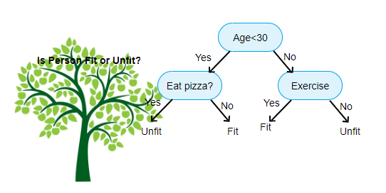
- Summarize what a decision tree algorithm does.
Series of yes and no questions, which it used to determine how to group the data. Here is the algorithm given in the book:
- Loop through each column of the dataset in turn
- For each column, loop through each possible level of that column in turn
- Try splitting the data into two groups, based on whether they are greater than or less than that value (or if it is a - categorical variable, based on whether they are equal to or not equal to that level of that categorical variable)
- Find the average sale price for each of those two groups, and see how close that is to the actual sale price of each of the items of equipment in that group. That is, treat this as a very simple “model” where our predictions are simply the average sale price of the item’s group
- After looping through all of the columns and possible levels for each, pick the split point which gave the best predictions using our very simple model
- We now have two different groups for our data, based on this selected split. Treat each of these as separate datasets, and find the best split for each, by going back to step one for each group
- Continue this process recursively, and until you have reached some stopping criterion for each group — for instance, stop splitting a group further when it has only 20 items in it.
- Why is a date different from a regular categorical or continuous variable, and how can you preprocess it to allow it to be used in a model?
Dates are different from other cetegorical/continuous data (Ex: some are holidays). Therefore, we can generate many different categorical features about the given date (ex: Is it the end of the month?) - Should you pick a random validation set in the bulldozer competition? If no, what kind of validation set should you pick?
You should not because here the date plays a major part as the test set contains data of the last 2 weeks. Therefore, we should split the data by the dates and include the later dates in the validation set. - What is pickle and what is it useful for?
Allows you so save any Python object as a file. - How are
mse,samples, andvaluescalculated in the decision tree drawn in this chapter?
By traversing the tree (based on answering questions about the data), we reach the nodes that tell us the average value of the data in that group. - How do we deal with outliers, before building a decision tree?
We can use random forest. But in this case we don’t use a random forest to predict our actual dependent variable. Instead we try to predict whether a row is in the validation set, or the training set. - How do we handle categorical variables in a decision tree?
We convert it into a numerical value that references the vocab. - What is bagging?
Training multiple models on random subsets of the data, and use the ensemble of models for prediction. - What is the difference between
max_samplesandmax_featureswhen creating a random forest?
max_samples defines how many rows of the tabular dataset we use for each decision tree.
max_features defines how many columns of the tabular dataset we use for each decision tree. - If you increase
n_estimatorsto a very high value, can that lead to overfitting? Why or why not?
No as the trees are independent of one another. - In the section "Creating a Random Forest", just after <
>, why did preds.mean(0)give the same result as our random forest?</strong>
Because much like the Random Forest that took the mean of the ensemble, we stacked all the dicision trees and took the mean across all the trees (dim=0).</li>- What is "out-of-bag-error"?
The OOB error is a way of measuring prediction error on the training set by only including in the calculation of a row's error trees where that row was not included in training. This allows us to see whether the model is overfitting, without needing a separate validation set.- Make a list of reasons why a model's validation set error might be worse than the OOB error. How could you test your hypotheses?
</ol>
Overfitting
Validation has different distributionOne way you can solve the distribution problem is by checking the standard deviation on the predictions.
- Explain why random forests are well suited to answering each of the following question:
- How confident are we in our predictions using a particular row of data?
Check the standard deviation on the predictions. - For predicting with a particular row of data, what were the most important factors, and how did they influence that prediction?
Check how the prediction changes as it goes through the tree, adding up the contributions from each split/feature. Use waterfall plot to visualize. - Which columns are the strongest predictors?
This is done by using featureimportance - How do predictions vary as we vary these columns?
Partial dependence plots
- How confident are we in our predictions using a particular row of data?
- What's the purpose of removing unimportant variables?
Improve model as its more interpertable with less clutering. Also, sometimes unnessary data can scew the prediction. - What's a good type of plot for showing tree interpreter results?
Waterfall plot - What is the "extrapolation problem"?
This was a demonstration of how a random forests cannot predict outside the domain of the training data. However, NN can generalize better due to their linear layers. - How can you tell if your test or validation set is distributed in a different way than your training set?
We can do so by training a model to classify if the data is training or validation data. If the data is of different distributions (out-of-domain data), then the model can properly classify between the two datasets. - Why do we ensure
saleElapsedis a continuous variable, even although it has less than 9,000 distinct values?
We want to make this a continuous variable as we want our model to determine future sales. - What is "boosting"?
We train a model that underfits the dataset, and train subsequent models that predicts the error of the original model. We then add the predictions of all the models to get the final prediction. - How could we use embeddings with a random forest? Would we expect this to help?
Instead of passing raw categorical columns, we can pass entity embeddings into the random forest model: This is better as embedding contain better representations of the features and will, in turn, improve the performance. - Why might we not always use a neural net for tabular modeling?
We might not use them because they are harder and longer to train.
</div>- Pick a competition on Kaggle with tabular data (current or past) and try to adapt the techniques seen in this chapter to get the best possible results. Compare your results to the private leaderboard.
Completed, see https://usama280.github.io/PasteBlogs/ (Tabular on Lesson 8) - Implement the decision tree algorithm in this chapter from scratch yourself, and try it on the dataset you used in the first exercise.
- Use the embeddings from the neural net in this chapter in a random forest, and see if you can improve on the random forest results we saw.
Completed, see https://usama280.github.io/PasteBlogs/ (EmbeddingRandomForest) - Explain what each line of the source of
TabularModeldoes (with the exception of theBatchNorm1dandDropoutlayers).
- What is "out-of-bag-error"?